Worked example NIST/SEMATECH dataset Not your current analysis

Distribution Identification → Normal Capability

Oxide film thickness in a semiconductor furnace

Follow one published industrial dataset from file preparation through distribution assessment, stability diagnostics and capability indices. The example explains the calculations without applying customer- or OEM-specific acceptance criteria.

Download example CSV Open Distribution Identification Open Normal Capability

Published dataset

Process and study structure

The data come from the NIST/SEMATECH furnace case study. A semiconductor manufacturing process grows an oxide film on silicon wafers. The study records film thickness across 21 process runs, four furnace zones and two wafers in each zone.

ResponseFilm thickness

UnitÅ (ångström)

Observations168

Study structure21 × 4 × 2

Specification460–660 Å

Target560 Å

Reading the structure: one run contains eight measurements: four furnace zones × two wafers. The original row order is therefore meaningful and must be preserved.

Input preparation

One readable file for both tools

CSV preview

run	zone	wafer	thickness
1	1	1	546
1	1	2	540
1	2	1	566
1	2	2	564
1	3	1	577
1	3	2	546
1	4	1	543
1	4	2	529

Preview: the first of 21 runs.

Column dictionary

run: Process run and proposed rational subgroup.
zone: One of four positions inside the furnace.
wafer: One of two measured wafers in each zone.
thickness: Numeric response used by both tools, in Å.

Distribution Identification Select measurement column: thickness

The remaining columns preserve traceability but are not fitted.

Normal Capability Select thickness; subgroup size: 8

Keep the file in acquisition order so every eight rows form one run.

Part A

Tool 1

Distribution Identification

Assess plausible probability models before capability calculations.

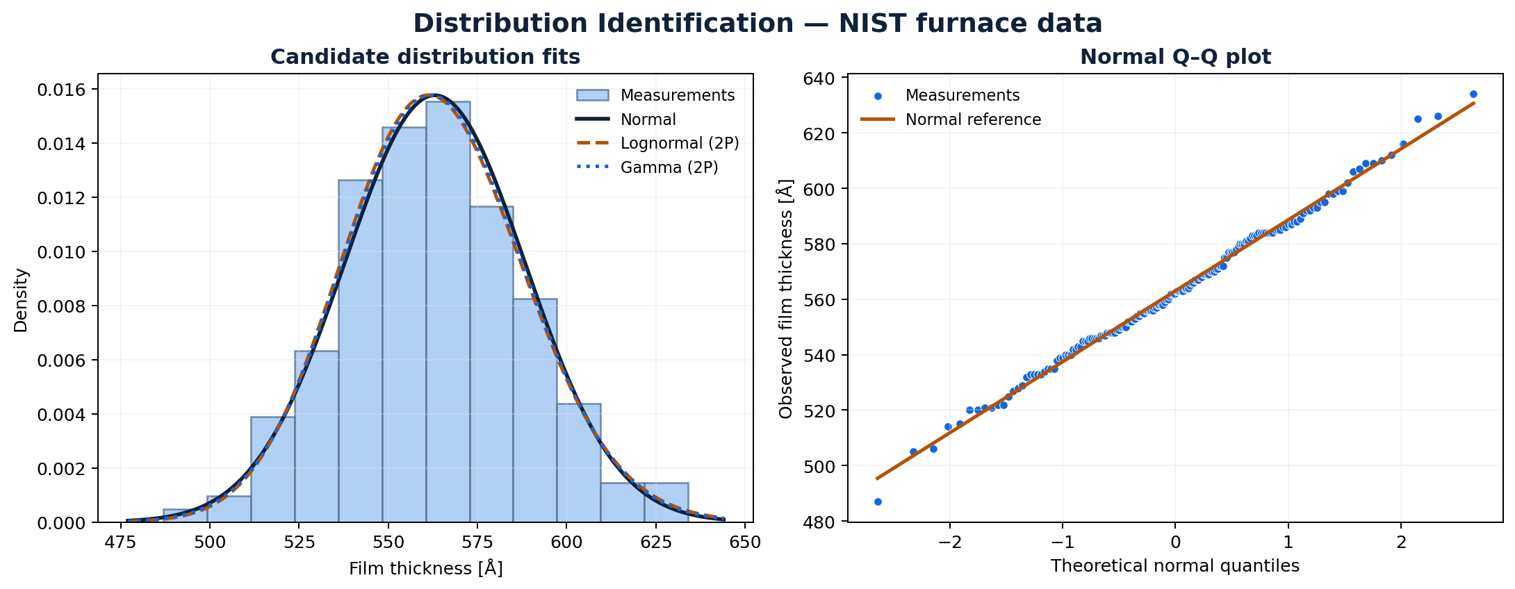
The question is not “Which distribution appears in the first row?” but “Which models describe the observed data adequately for the intended use?” QualityFirst ranks the evaluated candidates by the Anderson–Darling A² statistic and reports BIC as supporting information.

Histogram with normal, lognormal and gamma fits beside a normal Q-Q plot — The leading fitted curves almost overlap. The Q–Q plot provides a separate visual check of the normal working model.

Leading QualityFirst fits

Rank	Distribution	A²	BIC
1	Lognormal (2P)	0.2217	1572.782
2	Gamma (2P)	0.2230	1572.631
3	Lognormal (3P)	0.2289	1577.714
4	Gamma (3P)	0.2289	1577.716
5	Normal	0.2479	1572.681

How to read the result

Lower A² indicates a closer fit among the evaluated models.
The A² differences among the leading models are small.
The two-parameter BIC values are also almost indistinguishable.
Process knowledge and diagnostic plots remain part of model selection.

The normal model is retained as a transparent working model for the next section. Its dedicated normality test gives A² = 0.2495 and p = 0.7427; the available data do not provide evidence against normality at α = 0.05.

Do not turn rank into certainty. The table compares fitted candidates; it does not prove that the first model is the true population distribution. Here, several curves describe the central body of the data almost equally well.

Part A conclusion Working model retained: Normal distribution

The model is now carried into a capability analysis that also preserves the process sequence and subgroup structure.

Continue to Part B · Normal Capability ↓

Part B

Tool 2

Normal Capability

Evaluate stability, within variation and overall performance.

LSL460 Å

Target560 Å

USL660 Å

Subgroup size8

Subgroups21

First check: process stability

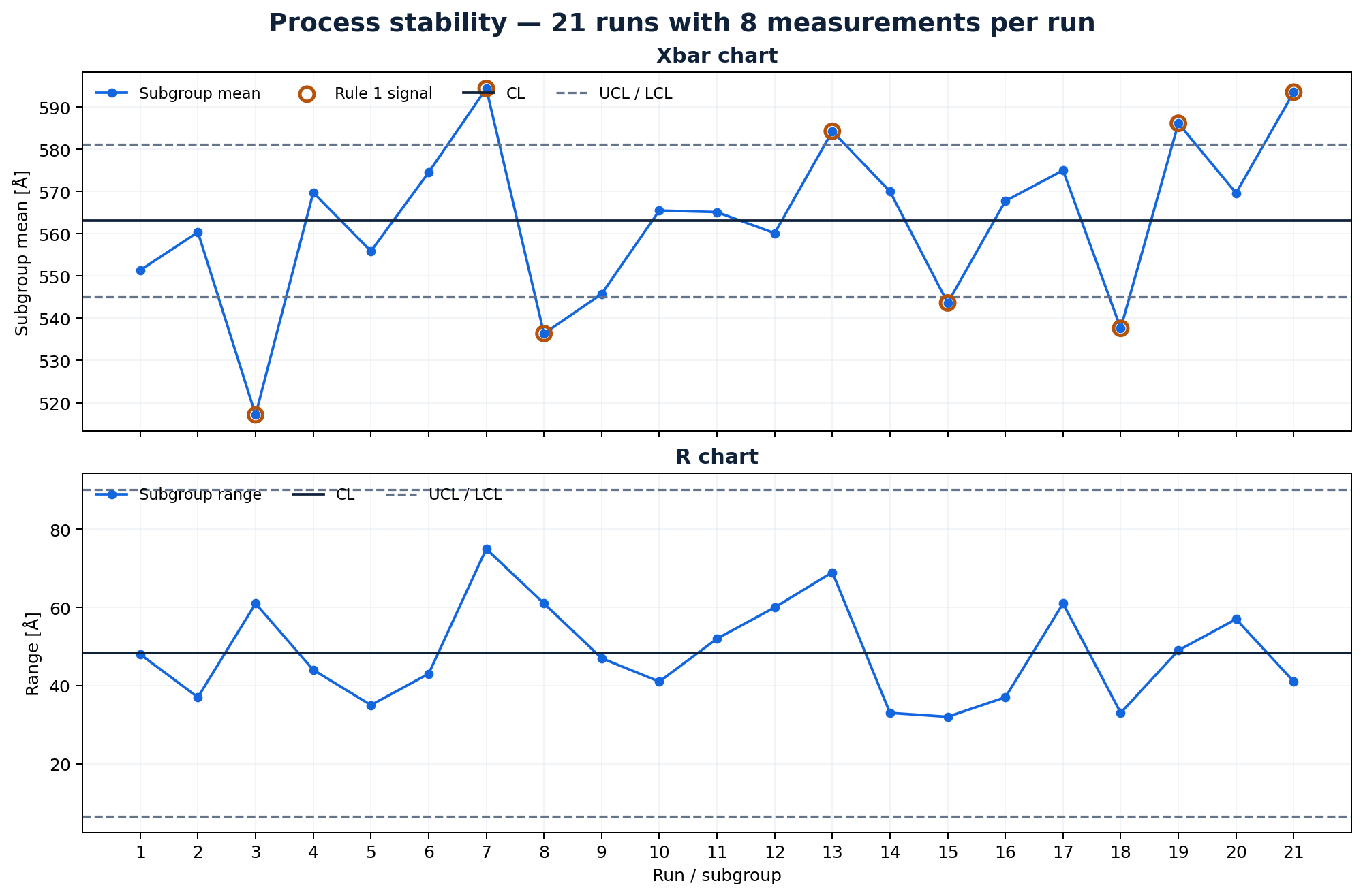
The Xbar–R chart evaluates the acquisition sequence before the capability indices are treated as a description of predictable future performance. QualityFirst currently evaluates Rule 1: a point outside the three-sigma control limits.

Xbar and R control charts for 21 furnace runs — Xbar signals occur in runs 3, 7, 8, 13, 15, 18, 19 and 21. The R chart has no Rule 1 signal.

Subgroup assumption: each run is treated as one subgroup. Its within-subgroup variation includes the four furnace zones and the two wafers measured in each zone. A different process question could require a different rational subgroup definition.

Variation estimates

N	168
Mean	563.03571 Å
Median	562.50000 Å
StDev Within	16.99366 Å
StDev Overall	25.38468 Å

Control limits

Statistic	Xbar	R
UCL	581.0818	90.1821
CL	563.0357	48.3810
LCL	544.9896	6.5798

Capability and performance indices

Within variation

Cp1.9615

Cpk1.9020

Cpl2.0211

Cpu1.9020

Estimated non-conformance: 0.01 ppm

Overall variation

Pp1.3131

Ppk1.2733

Ppl1.3530

Ppu1.2733

Estimated non-conformance: 91.43 ppm

NIST published reference “Cp” 1.313 · “Cpk” 1.273

These values match QualityFirst Pp and Ppk after rounding because the NIST reference calculation uses the overall sample standard deviation. QualityFirst reserves Cp and Cpk for the within-subgroup estimate, so the labels differ even though the comparable numerical results agree.

Interpretation warning: the gap between within and overall variation is consistent with the Xbar signals. The indices describe this dataset under stated assumptions; they are not presented here as an OEM acceptance decision.

Neutral conclusion

What this example demonstrates

Preserve structure. Run, zone and wafer identifiers explain how the measurements were acquired.
Read fit evidence together. Ranking, BIC, fitted curves, Q–Q behavior and process knowledge serve different purposes.
Normality is not stability. A plausible normal model can coexist with clear Xbar signals.
Know the sigma estimate. Cp/Cpk and Pp/Ppk answer different questions when within and overall variation differ.
Keep acceptance external. Customer and OEM rules must be applied separately to the documented result.

Reproducibility

Sources

QualityFirst calculations use the 168 observations in the published row order. Displayed values are rounded for readability; calculations use unrounded values.